PostgreSQL Performance Tuning: Optimize Your Database Server

A guide to improving database capabilities, from hardware to PostgreSQL query optimization
This document introduces tuning PostgreSQL and EDB Postgres Advanced Server (EPAS) versions 10 to 13. The system used is the RHEL family of Linux distributions, version 8. These are only general guidelines, and actual tuning details will vary by workload, but they should provide a good starting point for most deployments.
When tuning, we start with the hardware and work our way up the stack, finishing with the application's SQL queries. The workload-dependent aspect of tuning gets higher as we move up the stack, so we begin with the most general aspects and move on to the most workload-specific aspects.
Introduction to Postgres Tuning and Tooling
Getting the most out of PostgreSQL
Postgres tuning refers to the process of optimizing the performance and efficiency of PostgreSQL databases through careful adjustments of various configuration settings. This involves fine-tuning parameters related to memory usage, CPU allocation, disk I/O and query execution to ensure the database operates at its peak potential. With performance tuning, your system benefits from:
- Increased ability to handle more transactions per second, reducing latency and improving the overall user experience.
- More efficient use of system resources such as memory and CPU, preventing performance bottlenecks and reducing operational costs.
- Scalability, ensuring consistent performance under increased load.
- Reduced risk of crashes and failures and higher availability and reliability of your applications.
There are many tools available in the market to facilitate the management, monitoring and optimization of PostgreSQL databases. For example:
- pgAdmin, a powerful, open source management tool that provides a graphical interface for managing PostgreSQL databases.
- pgTune, which analyzes your system's resources and recommends configuration settings tailored to your environment.
- PgBouncer, Prometheus, and Grafana, which offer real-time monitoring and alerting for PostgreSQL databases, helping to identify performance issues and trends.
- Extensions like pg_stat_statements and pgBadger that help in tracking and analyzing query performance, providing insights into slow queries and potential optimizations.
With a plethora of information and tools available for PostgreSQL, how do you know the right approach, methodology or tool to use at any given time? EnterpriseDB (EDB) can help take the guesswork out of PostgreSQL optimization. No one else knows PostgreSQL as well as the experts at EDB. With more open source contributions to PostgreSQL than any other company, EDB is uniquely positioned to provide unparalleled expertise. Take advantage of the EDB Interactive Postgres Tuning Guide to finely configure your PostgreSQL database server to meet your organization’s specific needs.
Fundamentals of Postgres Tuning
Learn more about the basic principles and methodologies of tuning PostgreSQL
Four Key Parameters and Settings to Fine-tune for Better Efficiency and Responsiveness
- Memory settings
- shared_buffers: The shared_buffers parameter controls the amount of memory PostgreSQL uses for shared memory buffers. Properly setting this parameter is crucial for performance, as it determines how much data can be cached in memory. Typically, setting shared_buffers to 25-40% of the total system memory is recommended for most workloads.
- work_mem: The work_mem setting affects the memory allocated for complex queries and sorting operations. Higher values can improve performance for large sorts and hash joins, but setting it too high can lead to excessive memory usage, particularly in environments with many concurrent queries.
- WAL (Write-Ahead Logging) settings
- wal_buffers, checkpoint_segments: These settings impact the performance and durability of your PostgreSQL database. wal_buffers determines the amount of shared memory used for write-ahead logs, while checkpoint_segments affects the frequency of checkpoints. Proper configuration can reduce I/O contention and enhance write performance.
- Autovacuum settings
- Autovacuum is essential for maintaining table health by preventing transaction ID wraparound and reclaiming storage from dead tuples.
Key parameters:- autovacuum_naptime: Controls the frequency of autovacuum runs. A lower value can help maintain table health but might increase system load.
- autovacuum_vacuum_threshold and autovacuum_analyze_threshold: These parameters determine when autovacuum should perform vacuuming and analyzing operations based on the number of row updates and inserts.
- Query planner settings
- random_page_cost, seq_page_cost: These settings influence the PostgreSQL query planner’s decisions. random_page_cost is the cost of a non-sequential page fetch, while seq_page_cost is the cost of fetching a sequential page. Tuning these values helps the planner make more efficient query execution plans, improving performance.
Understanding Database Workload and Performance Metrics
Different types of workloads have distinct characteristics and tuning requirements. Identify the nature of your workload and monitor critical performance metrics to tailor your tuning efforts to specific needs and demands.
Here is a side-by-side comparison table of the two types of workloads with key metrics to monitor (table below):
Aspect | OLTP (Online Transaction Processing) | OLAP (Online Analytical Processing) |
Primary Focus | Fast transaction processing with high concurrency | Complex queries and data analysis |
Key Benefits | Optimized indexing and fast writes | Efficient read operations and large memory allocations |
Transactions Per Second(TPS) | High TPS is critical | Generally lower TPS compared to OLTP |
Query Execution Times | Typically short, focused on quick insert/update/delete operations | Longer execution times due to complex queries |
Disk I/O Operations | Optimized for write-heavy operations | Optimized for read-heavy operations |
CPU Usage and Memory Consumption | Requires balanced CPU and memory resources to handle high concurrency | Requires significant memory for efficient data processing and analysis |
*Key metrics definitions
- Transactions Per Second(TPS): Measures the number of transactions processed per second, a critical metric for OLTP systems.
- Query execution times: Monitoring execution times helps identify slow queries that need optimization.
- Disk I/O operations: High disk I/O can indicate inefficient queries or insufficient memory settings.
- CPU usage and memory consumption: Balancing CPU and memory resources is essential for maintaining performance and preventing system overloads.
Common PostgreSQL Tuning Practices and Their Impact
- Indexing
- Indexes improve query performance by allowing faster data retrieval. PostgreSQL supports several types of indexes, each suited for different use cases:
- B-tree: The default and most commonly used index type, B-tree is versatile and efficient for a wide range of queries, particularly those involving equality and range comparisons. Suitable for columns used in WHERE clauses with equality (=) and range operators (<,>, <=,>=). It's also effective for ORDER BY and GROUP BY clauses.
- Hash: Designed for very fast equality comparisons, they store the hash value of the indexed column, allowing rapid lookups. Ideal for columns where queries involve equality checks (=). However, they are not suitable for range queries.
- GIN (generalized inverted index): Useful for indexing composite values, such as arrays, full-text search and JSONB data, they store a mapping between keys and their associated row identifiers.
- GiST (generalized search tree): Flexible and can handle a variety of data types and operations, the support indexing of geometric shapes, ranges, and full-text search. They can be tailored for various types of queries by defining custom strategies.
- Query Optimization
- By optimizing queries, you can reduce execution times, minimize resource consumption, and improve overall database performance. This process involves analyzing and refining SQL statements to ensure they are executed in the most efficient manner possible. Key techniques include:
- Using EXPLAIN: The EXPLAIN command provides a detailed description of how PostgreSQL executes a query. By running EXPLAIN, you can see the execution plan, which outlines the steps PostgreSQL takes to retrieve the desired data. This plan includes information about the access methods used (e.g., sequential scans, index scans), join methods, and estimated costs. Understanding the execution plan helps you identify inefficiencies in your query and provides insights into possible optimizations.
- Using ANALYZE: The ANALYZE command goes a step further by actually executing the query and providing runtime statistics. When combined with EXPLAIN, it shows both the estimated and actual execution times, allowing you to compare the planner's expectations with reality. This helps in identifying discrepancies and understanding where the query might be optimized further.
- VACUUM and ANALYZE
- VACUUM and ANALYZE are two essential maintenance operations that help to reclaim storage, update statistics, and prevent issues related to transaction ID wraparound.
- VACUUM: There are two types – VACUUM FULL, which completely rewrites the table, reclaiming space and returning it to the operating system, and Standard VACUUM, which reclaims space and makes it available for reuse, but does not return the space to the operating system. This is often used to maintain table health and performance.
- ANALYZE: This is used primarily to update statistics and improve query performance. Regularly running ANALYZE helps maintain accurate statistics.
What Are Essential Tools for PostgreSQL DBA?
Explore the various tools available to assist in various aspects of database administration, from performance monitoring and analysis to routine maintenance and automated tuning
pgAdmin
pgAdmin is a powerful, open source graphical management tool for PostgreSQL. It provides a user-friendly interface for managing databases, executing queries, and performing administrative tasks.
Key features
- Comprehensive database management: Offers tools for creating, modifying, and deleting databases, tables, and other database objects.
- Query tool: Allows users to write and execute SQL queries, view results, and optimize queries.
- User management: Facilitates the management of user roles and permissions.
- Backup and Restore: Provides features for backing up and restoring databases.
pgTune
pgTune is a configuration tuning tool for PostgreSQL that analyzes your system’s resources and recommends optimal configuration settings. It eliminates the complexity of manually tuning PostgreSQL configuration parameters and ensures that your database setup is optimized for the available hardware resources, improving overall performance.
Key features
- Automated configuration suggestions: Analyzes hardware resources (memory, CPU, disk) and provides tailored configuration recommendations.
- Easy integration: Generates configuration files that can be easily applied to PostgreSQL instances.
Prometheus and Grafana
Prometheus is an open source monitoring system, while Grafana is a powerful visualization tool. Together, they provide comprehensive monitoring and visualization for PostgreSQL databases. What you get is total visibility into your database performance with real-time metrics and custom dashboards.
Key features
- Real-time monitoring: Collects and stores metrics from PostgreSQL and other systems in real-time.
- Custom dashboards: Grafana enables the creation of custom dashboards to visualize metrics and monitor database health.
- Alerting: Prometheus provides alerting capabilities based on the metrics collected.
pgBadger
pgBadger is a fast PostgreSQL log analyzer that generates detailed reports on database performance. Not only does it simplify the analysis of PostgreSQL logs, offering actionable insights into performance issues, it also helps identify slow queries and other bottlenecks through detailed reports.
Key features
- Log analysis: Parses PostgreSQL logs and generates performance reports.
- Visual reports: Provides graphical reports on various performance metrics, including slow queries and connections.
pg_autovacuum
pg_autovacuum is a built-in PostgreSQL daemon that automates the execution of VACUUM and ANALYZE operations. It ensures database health by regularly reclaiming storage and updating statistics and reduces the need for manual intervention by running auto maintenance tasks.
Key features
- Automatic maintenance: Runs VACUUM and ANALYZE operations automatically based on database activity.
- Configurable: Parameters can be adjusted to control the frequency and behavior of maintenance tasks.
What Value Do Enterprises Get Using These Tools?
Enterprise-Grade Tools
Enhanced security, compliance, performance, and availability to ensure Postgres is ready for mission-critical workloads.
Secure Supply Chain
Increase assurance with a secure, open source supply chain. Use only trusted repositories with full commercial support for PostgreSQL extensions.
Advanced Analytics
Ensure efficient database management and monitoring to identify insights into trends, patterns, and correlations for better decision-making.
Key Hardware Components and Considerations in PostgreSQL Tuning and Tooling
Bare metal
A few things need to be considered when designing a bare metal server for PostgreSQL. These are CPU, RAM, disk, and the network card in some cases.
CPU
The right CPU may be crucial to PostgreSQL performance. CPU speed will be important when dealing with larger data, and CPUs with larger L3 caches will boost performance. For OLTP performance, having more and faster cores will help the operating system and PostgreSQL be more efficient. Meanwhile, using CPUs with larger L3 caches is suitable for larger data sets.
What is an L3 cache? CPUs have at least two caches: L1 (a.k.a. primary cache) and L2 (a.k.a. secondary cache). L1 is the smallest and fastest cache embedded into the CPU core. L2 is a bit slower than L1 but larger and is used to feed L1.
Unlike L1 and L2 caches, which are unique to each core, the L3 cache is shared across all available cores. L3 is slower than L1 and L2 but is still faster than RAM. A larger L3 cache will boost CPU performance while dealing with a larger data set. This will also benefit PostgreSQL for parallel queries.
RAM
RAM is the cheapest among the hardware and the best for PostgreSQL performance. Operating systems utilize the available memory and try to cache as much data as possible. More caching will result in less disk I/O and faster query times. When buying new hardware, add as much RAM as possible, as adding more in the future will be more expensive financially and technically. It will require downtime unless you have a system with hotswap RAM. Multiple PostgreSQL parameters will be changed based on the available memory, which are mentioned below.
Disk
If the application is I/O-bound (read and/or write-intensive), a faster drive set will improve performance significantly. There are multiple solutions available, including NMVe and SSD drives.
The first rule of thumb is to separate the WAL disk from the data disk. WAL may be a bottleneck on write-intensive databases, so keeping WAL on a separate and fast drive will solve this problem. Always use at least RAID 1, though there are some cases where you may need RAID 10 if the database is writing a lot.
Using separate tablespaces and drives for indexes and data will also increase performance, especially if PostgreSQL runs on SATA drives. This is usually not needed for SSD and NVMe drives. We suggest using RAID 10 for data.
Please refer to the “Optimizing File System” section for more information about optimizing drives. In addition, this blog discusses the storage and RAID options that can be used with PostgreSQL.
Network card
Even though network cards seem irrelevant to PostgreSQL performance, when the data grows a lot, faster or bonded network cards will also speed up base backups.
Virtual Machines
Virtual machines have a slight performance deficit compared to bare metal servers due to the virtualization layer. The available CPU and disk I/O will also decrease due to shared resources.
There are a few tips to get better performance out of PostgreSQL in VMs:
- Pin the VM to specific CPUs and disks. That will eliminate or limit the performance bottleneck because of other VMs running on the host machine.
- Pre-allocate the disks before installation. That will prevent the host from allocating the disk space during database operations. You can change these two parameters in postgresql.conf if you cannot do this:
- Disable the wal_recycle parameter in postgresql.conf. By default, PostgreSQL recycles the WAL files by renaming them. However, on Copy-On-Write (COW) filesystems, creating new WAL files may be faster, so disabling this parameter will help in the VMs.
- Disable the wal_init_zero parameter in postgresql.conf. By default, WAL space is allocated before WAL records are inserted. This will slow down WAL operations on COW filesystems. Disabling this parameter will disable this feature, helping VMs to perform better. If set to off, only the final byte is written when the file is created so that it has the expected size.
Tuning the System
Tuning the PostgreSQL operating system gives you extra opportunities for better performance. As the introduction notes, this guide focuses on tuning PostgreSQL for the Red Hat Enterprise Linux (RHEL) family.
tuned daemon
Most of the tuning on RHEL is done with the tuned daemon. This daemon adapts the operating system to perform better for the workload.
Note that the commands shown below are for RHEL 8. If you're using RHEL 7, use the yum command wherever dnf is shown in the examples.
The tuned daemon comes installed by default. If it does not (perhaps due to the configuration of kickstart files), install it with:
dnf -y install tunedAnd enable it with:
systemctl enable --now tunedtuned helps sysadmins to change kernel settings quickly and dynamically, and they no longer need to make changes in /etc/sysctl – this is done via tuned.
tuned comes with a few predefined profiles. You can get the list using the tuned-adm list command. The RHEL installer will pick up a good default based on the environment. The bare metal default is throughput-performance, which aims at increasing throughput. You can run the following command to see what tuned daemon will recommend after assessing your system:
tuned-adm recommendUse the command below to see the preconfigured value:
tuned-adm active
Current active profile: virtual-guest
However, the defaults may slow down PostgreSQL; they may prefer power saving, which will slow down CPUs. Similar arguments are valid for network and I/O tuning as well. To solve this problem, we will create our own profile for PostgreSQL performance.
Creating a new profile is relatively easy. Let’s call this profile edbpostgres. Run these commands as root:
#  This directory name will also be the
# name of the profile:
mkdir /etc/tuned/edbpostgres
# Create the profile file:
echo "
[main]
summary=Tuned profile for EDB PostgreSQL Instances
[bootloader]
cmdline=transparent_hugepage=never
[cpu]
governor=performance
energy_perf_bias=performance
min_perf_pct=100
[sysctl]
vm.swappiness = 10
vm.dirty_expire_centisecs = 500
vm.dirty_writeback_centisecs = 250
vm.dirty_ratio = 10
vm.dirty_background_ratio = 3
vm.overcommit_memory=0
net.ipv4.tcp_timestamps=0

[vm]
transparent_hugepages=never
" > /etc/tuned/edbpostgres/tuned.conf
The lines that include [ and ] are called tuned plugins and are used to interact with the given part of the system.
Let’s examine these parameters and values:
- [main] plugin includes summary information and can also include values from other tuned profiles with include statements.
- [cpu] plugin includes settings around CPU governor and CPU power settings.
- [sysctl] plugin includes the values that interact with procfs.
- [vm] and [bootloader] plugins enable/disable transparent huge pages (the bootloader plugin will help us to interact with GRUB command line parameters).
With these changes, we aim to achieve the following:
- CPUs will not enter power-saving modes (PostgreSQL won’t suffer from random performance slowdowns).
- Linux will be much less likely to swap.
- The kernel will help Postgres to flush dirty pages, reducing the load of bgwriter and checkpointer.
- The pdflush daemon will run more frequently.
- It is good practice to turn TCP timestamps off to avoid or at least reduce spikes caused by timestamp generation.
- Disabling transparent huge pages is a great benefit to PostgreSQL performance.
To enable these changes, run this command:
tuned-adm profile edbpostgresThis command may take some time to complete.
To disable transparent huge pages completely, run this command:
grub2-mkconfig -o /boot/grub2/grub.cfgand reboot your system:
systemctl start reboot.targetOptimizing the File System
Another tuning point is disks. PostgreSQL does not rely on atime (the timestamp at which the file was last accessed) for data files, so disabling them will save CPU cycles.
Open /etc/fstab and add noatime near the defaults value for the drive where PostgreSQL data and WAL files are kept.
/dev/mapper/pgdata-01-data /pgdata xfs defaults,noatime 1 1To activate it immediately, run:
mount -o remount,noatime,nodiratime /pgdataThese suggestions are good for a start, and you need to monitor both the operating system and PostgreSQL to gather more data for finer tuning.
Huge Pages
By default, the page size on Linux is 4KB. A typical PostgreSQL instance may allocate many GBs of memory, leading to potential performance problems due to the small page size. Also, since these pages will be fragmented, mapping them for large data sets requires extra time.
Enabling huge pages on Linux will boost PostgreSQL performance as it will allocate large blocks (huge pages) of memory altogether.
By default, huge pages are not enabled on Linux, which is also suitable for PostgreSQL’s default huge_pages setting try, which means “use huge pages if available on the OS, otherwise no”.
There are two aspects to setting up huge pages for PostgreSQL: Configuring the OS and configuring PostgreSQL.
First, find out how many huge pages your system needs for PostgreSQL. When a PostgreSQL instance is started, the postmaster creates a postmaster.pid file in $PGDATA. You can find the pid of the main process there:
$ head -n 1 $PGDATA/postmaster.pid
1991
Now, find VmPeak for this instance:
$ grep -i vmpeak /proc/1991/status
VmPeak: 8823028 kB
Tip: If running more than one PostgreSQL instance on the same server, calculate the sum of all VmPeak values in the next step.
Let’s confirm the huge page size:
$ grep -i hugepagesize /proc/meminfo
Hugepagesize: 2048 kB
Finally, let’s calculate the number of huge pages that the instance(s) will need:
8823028 / 2048 = 4308.12
The ideal number of huge pages is slightly higher than this value – just marginally. If you increase this value too much, processes that need small pages and space in the OS will fail to start. This may even result in the operating system failing to boot or other PostgreSQL instances on the same server failing to start.
Now edit the tuned.conf file created above, and add the following line to the [sysctl] section:
vm.nr_hugepages=4500and run this command to enable new settings:
tuned-adm profile edbpostgresNow you can set
huge_pages=onin postgresql.conf , and (re)start PostgreSQL.
We also need to ensure that the tuned service starts before the PostgreSQL service and after rebooting. So, the next step would be to edit unit file:
systemctl edit postgresql-13.serviceand add these two lines:
[Unit]
After=tuned.service
Run:
systemctl daemon-reloadfor the changes to take effect.
PostgreSQL Performance Tuning Starting Points
The following configuration options should be changed from the default values in PostgreSQL. Other values can significantly affect performance but are not discussed here as their defaults are already considered optimal.
Configuration and Authentication
max_connections
The optimal number for max_connections is roughly four times the number of CPU cores. This formula often gives a minimal number, which doesn’t leave much room for error. The recommended number is the GREATEST(4 x CPU cores, 100). Beyond this number, a connection pooler such as pgbouncer should be used.
It is important to avoid setting max_connections too high as it will increase the size of various data structures in Postgres, wasting CPU cycles. Conversely, we must also ensure that enough resources are allocated to support the required workload.
Resource Usage
shared_buffers
This parameter has the most variance of all. Some workloads work best with minimal values (such as 1GB or 2GB), even with huge database volumes. Other workloads require large values. The LEAST(RAM/2, 10GB) is a reasonable starting point.
This formula has no specific reason beyond the PostgreSQL community’s years of collective wisdom and experience. Complex interactions between the kernel cache and shared_buffers make it nearly impossible to describe exactly why this formula generally provides good results.
work_mem
The recommended starting point for work_mem is ((Total RAM - shared_buffers)/(16 x CPU cores)). The rationale behind this formula is that if you have numerous queries risking memory depletion, the system will already be constrained by CPU capacity. This formula provides for a relatively large limit for the general case.
It can be tempting to set work_mem to a higher value, but this should be avoided as the amount of memory specified here may be used by each node within a single query plan. Thus, a single query could use multiple work_mem in total, for example, in a nested string of hash joins.
maintenance_work_mem
This determines the maximum amount of memory used for maintenance operations like VACUUM, CREATE INDEX, ALTER TABLE ADD FOREIGN KEY, and data-loading operations. These may increase the I/O on the database servers while performing such activities, so allocating more memory to them may lead to these operations finishing more quickly. A value of 1GB is a good start since these are commands explicitly run by the DBA.
autovacuum_work_mem
Setting maintenance_work_mem to a high value will also allow autovacuum workers to use that much memory each. A vacuum worker uses 6 bytes of memory for each dead tuple it wants to clean up, so a value of just 8MB will allow for about 1.4 million dead tuples.
effective_io_concurrency
This parameter is used for read-ahead during certain operations and should be set to the number of disks used to store the data. It was originally intended to help Postgres understand how many reads would likely occur in parallel when using striped RAID arrays of spinning disks. However, improvements have been observed by using a multiple of that number, likely because good quality RAID adaptors can re-order and pipeline requests for efficiency. For SSD disks, set this value to 200 as their behavior differs from spinning disks.
Write-Ahead Log
wal_compression
When this parameter is on, the PostgreSQL server compresses a full-page image written to WAL when full_page_writes is on or during a base backup. Set this parameter to on, as most database servers will likely be bottlenecked on I/O rather than CPU.
wal_log_hints
This parameter is required to use pg_rewind. Set it to on.
wal_buffers
This controls the space available for backends to write WAL data in memory so the WALWriter can then write it to the WAL log on disk in the background. WAL segments are 16MB each by default, so buffering a segment is inexpensive memory-wise. Larger buffer sizes were observed to have a potentially positive effect on testing performance. Set this parameter to 64MB.
checkpoint_timeout
Longer timeouts reduce overall WAL volume but make crash recovery slower. The recommended value is at least 15 minutes, but ultimately, the RPO of business requirements dictates what this should be.
checkpoint_completion_target
This determines the time in which PostgreSQL aims to complete a checkpoint. This means a checkpoint does not need to result in an I/O spike; instead, it aims to spread the writes over this fraction of the checkpoint_timeout value. The recommended value is 0.9 (which will become the default in PostgreSQL 14).
max_wal_size
A timeout for better performance and predictability should always trigger checkpoints. The max_wal_size parameter should be used to protect against running out of disk space by ensuring a checkpoint occurs when we reach this value to enable WAL to be recycled. The recommended value is half to two-thirds of the available disk space where the WAL is located.
archive_mode
Because changing this requires a restart, it should be set to on, unless you know you will never use WAL archiving.
archive_command
A valid archive_command is required if archive_mode is on. Until archiving is ready to be configured, a default of “: to be configured” is suggested.
The “:” primitive simply returns success on POSIX systems (including Windows), telling Postgres that the WAL segment may be recycled or removed. The to be configured is a set of arguments that will be ignored.
PostgreSQL Query Optimization
random_page_cost
This parameter gives the PostgreSQL optimizer a hint about the cost of reading a random page from disk, allowing it to decide when to use index scans vs. sequential scans. If using SSD disks, the recommended value is 1.1. For spinning disks, the default value is often adequate. This parameter should be set globally and per tablespace. If you have a tablespace containing historical data on a tape drive, you might want to set this very high to discourage random access; a sequential scan and a filter will likely be faster than using an index.
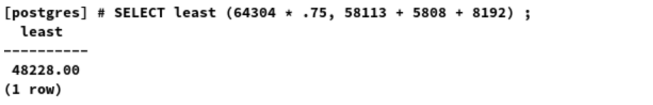
effective_cache_size
This should be set to the smaller value of either 0.75* total RAM amount, or the sum of buff/cache, free RAM, and shared buffers in the output of free command, and is used to give PostgreSQL a hint about how much total cache space is available. This refers to caches in main memory, not CPU cache.
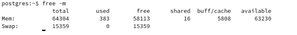
In this example, effective_cache_size will be least (64304 * .75, 58113 + 5808 + 8192) (assuming that shared_buffers is 8GB, so 48228 MB.
cpu_tuple_cost
Specifies the relative cost of processing each row during a query. Its default value is 0.01, but this is likely to be lower than optimal, and experience shows it should usually be increased to 0.03 for a more realistic cost.
Reporting and Logging
logging_collector
This parameter should be on if log_destination includes stderr or csvlog to collect the output into log files.
log_directory
If the logging_collector is on, this should be set to a location outside the data directory. This way, the logs are not part of base backups.
log_checkpoints
This should be set to on for future diagnostic purposes – in particular, to verify that checkpoints are happening by checkpoint_timeout and not by max_wal_size.
log_line_prefix
This defines the prefix format prepended to lines in the log file. The prefix should at least contain the time, the process ID, the line number, the user and database, and the application name to aid diagnostics.
Suggested value: '%m [%p-%l] %u@%d app=%a '
Don’t forget the space at the end!
log_lock_waits
Set to on. This parameter is essential in diagnosing slow queries.
log_statement
Set to ddl. In addition to leaving a basic audit trail, this will help determine when a catastrophic human error occurred, such as dropping the wrong table.
log_temp_files
Set to 0. This will log all temporary files created, suggesting that work_mem is incorrectly tuned.
timed_statistics (EPAS)
Controls timing data collection for the Dynamic Runtime Instrumentation Tools Architecture (DRITA) feature. When set to on, timing data is collected. Set this parameter to on.
Autovacuum
log_autovacuum_min_duration
Monitoring autovacuum activity will help with tuning it. Suggested value: 0, which will log all autovacuum activity.
autovacuum_max_workers
This is the number of workers that autovacuum has. The default value is 3 and requires a database server restart to be updated. Each table can have only one worker working on it, so increasing workers only helps in parallel and more frequent vacuuming across tables. The default value is low, so it is best to increase this value to 5 as a starting point.
autovacuum_vacuum_cost_limit
To prevent excessive load on the database server due to autovacuum, Postgres has imposed an I/O quota. Every read/write causes depletion of this quota, and once it is exhausted, the autovacuum processes sleep for a fixed time. This configuration increases the quota limit, increasing the amount of I/O that the vacuum can do. The default value is low; we recommend increasing this value to 3000.
Client Connection Defaults
idle_in_transaction_session_timeout
Sessions that remain idle in a transaction can hold locks and prevent vacuum. This timer will terminate sessions that remain idle in a transaction for too long, so the application must be prepared to recover from such an ejection.
Suggested value: 10 minutes if the application can handle it.
lc_messages
Log analyzers only understand untranslated messages. Set this to C to avoid translation.
shared_preload_libraries
Adding pg_stat_statements has a low overhead and high value. This is recommended but optional (see below).
PostgreSQL Performance Tuning Based on Workload Analysis
Finding Slow Queries
There are two main ways to find slow queries:
- The log_min_duration_statement parameter; and
- the pg_stat_statements module and extension.
The log_min_duration_statement parameter is a time setting (granularity milliseconds) that indicates how long a query must run before sending it to the log file. To get all the queries, set this to 0, but be warned: this can cause quite a lot of I/O!
Generally, this is set to 1s (one second), and all the queries are optimized as described below. Then, it is gradually lowered, and the process is repeated until a reasonable threshold is reached, and then kept there for ongoing optimization. What constitutes a reasonable threshold is dependent on your workload.
This technique is good for finding slow queries, but it isn’t the best. Imagine a query that takes 1 min to execute and runs every 10 minutes. Now, you have a query that takes 20ms to execute but runs 20 times per second. Which one is more important to optimize? Normalized to 10 minutes, the first query takes one minute of your server’s time, and the second takes four minutes. So, the second is more important than the first, but it will likely fly under your log_min_duration_statement radar.
Enter the pg_stat_statements module. One of its downsides is that it needs to be set in shared_preload_libraries, which requires a server restart. Fortunately, its overhead is so low, and the rewards so high, that we recommend always installing it in production.
What this module does is record every single (completed) query that the server executes, normalizes it in various ways such as replacing constants with parameters, and then aggregates “same” queries into a single data point with interesting statistics such as total execution time, number of calls, maximum and minimum execution time, total number of rows returned, total size of temporary files created, and more.
Two queries are considered the “same” if their normalized internal structures after parsing are the same. So SELECT * FROM t WHERE pk = 42; is the “same” query as SeLeCt * FrOm T wHeRe Pk=56; despite the value of pk being different.
To see the statistics collected by the pg_stat_statements module, you first need to install the pg_stat_statements extension with CREATE EXTENSION pg_stat_statements, creating a pg_stat_statements view.
A word about security. The module collects statistics from all queries to the server, regardless of which combination of users/databases they were run against. If desired, the extension can be installed in any database, even multiple databases. By default, any user can select from the view but are limited to only their queries (the same as with the pg_stat_activity view). Superusers and users granted to the pg_read_all_stats or pg_monitor roles can see all the contents.
EDB’s PostgreSQL Enterprise Manager (PEM) has an SQL Profiler that can display this nicely.
Rewriting Queries
Sometimes, rewriting parts of a query can drastically improve performance.
Naked columns
One very common mistake is writing something like this:
SELECT * FROM t
WHERE t.a_timestamp + interval ‘3 days’ < CURRENT_TIMESTAMP
Instead of this:
SELECT * FROM t
WHERE t.a_timestamp < CURRENT_TIMESTAMP - interval ‘3 days’
The results of these two queries will be the same; there is no semantic difference. However, the second one can use an index on t.a_timestamp, and the first one cannot. Keep the table columns “naked” on the left side and put all expressions on the right.
Never Use NOT IN with a Subquery
The IN predicate has two forms: x IN (a, b, c) and x IN (SELECT …). You can use either one for the positive version. For the negative, use the first. It’s because of how nulls are handled.
Consider:
demo=# select 1 in (1, 2);
?column?
----------
t
(1 row)
demo=# select 1 in (1, null);
?column?
----------
t
(1 row)
demo=# select 1 in (2, null);
?column?
----------
(null)
(1 row)
This shows that in the presence of nulls, the IN predicate will only return true or null – never false. It follows that NOT IN will only return false or null – never true!
When giving a list of constants like that, it is easy to spot when there are nulls and see that the query will never provide the desired results. But if you use the subquery version, it is not so easy to see. More importantly, even if the subquery result is guaranteed to have no nulls, Postgres won’t optimize it into an anti join. Use NOT EXISTS instead.
Using EXPLAIN (ANALYZE, BUFFERS)
If your query never terminates (at least before you lose patience and give up), you should contact an expert or become an expert to study the simple EXPLAIN plan. In all other cases, you must always use the ANALYZE option to optimize a query.
Bad estimates
The most common cause of bad performance is bad estimates. If the table statistics are not up to date, Postgres might predict only two rows will be returned when 200 rows will be returned. For just a scan, this is not important; it will take a little longer than predicted, but that’s it.
The real problem is the butterfly effect. If Postgres thinks a scan will produce two rows, it might choose a nested loop for a join against it. When it gets 200 rows, that’s a slow query, and if it knew there would be that many rows, it would have chosen a hash join or a merge join. Updating the statistics with ANALYZE can fix the problem.
Alternatively, you may have strongly correlated data the planner does not know about. You can solve this problem with CREATE STATISTICS.
External sorts
If there is insufficient work_mem for a sort operation, Postgres will spill to the disk. Since RAM is much faster than disks (even SSDs), this can cause slow queries. Consider increasing work_mem if you see this.
demo=# create table t (c bigint);
CREATE TABLE
demo=# insert into t select generate_series(1, 1000000);
INSERT 0 1000000 demo=# explain (analyze on, costs off) table t order by c;
                         QUERY PLAN
----------------------------------------------------------------------
Sort (actual time=158.066..245.686 rows=1000000 loops=1)
 Sort Key: c
 Sort Method: external merge Disk: 17696kB
 -> Seq Scan on t (actual
time=0.011..51.972 rows=1000000 loops=1)
Planning Time: 0.041 ms
Execution Time: 273.973 ms
(6 rows)

demo=# set work_mem to '100MB';
SET
demo=# explain (analyze on, costs off) table t order by c;
                         QUERY PLAN
----------------------------------------------------------------------
Sort (actual time=183.841..218.555 rows=1000000 loops=1)
 Sort Key: c
 Sort Method: quicksort Memory: 71452kB
 -> Seq Scan on t (actual time=0.011..56.573 rows=1000000 loops=1)
Planning Time: 0.043 ms
Execution Time: 243.031 ms
(6 rows)
The difference isn’t flagrant here because of the small dataset. Real-world queries can be much more noticeable. Sometimes, it is best to add an index to avoid the sort altogether.
To prevent pathological, runaway queries, set the temp_file_limit parameter. A query that generates this much in temporary files is automatically canceled.
Hash batches
Another indicator that work_mem is set too low is if a hashing operation is done in batches. In this next example, we set work_mem to its lowest possible setting before running the query. Then, we reset it and rerun the query to compare plans.
demo=# create table t1 (c) as select generate_series(1, 1000000);
SELECT 1000000
demo=# create table t2 (c) as select generate_series(1, 1000000, 100);
SELECT 10000
demo=# vacuum analyze t1, t2;
VACUUM
demo=# set work_mem to '64kB';
SET
demo=# explain (analyze on, costs off, timing off)
demo-# select * from t1 join t2 using (c);
                         QUERY PLAN
------------------------------------------------------------------
Gather (actual rows=10000 loops=1)
Workers Planned: 2
Workers Launched: 2
-> Hash Join (actual rows=3333 loops=3)
   Hash Cond: (t1.c = t2.c)
-> Parallel Seq Scan on t1 (actual rows=333333 loops=3)
-> Hash (actual rows=10000 loops=3)
   Buckets: 2048 Batches: 16 Memory Usage: 40kB
-> Seq Scan on t2 (actual rows=10000 loops=3)
Planning Time: 0.077 ms
Execution Time: 115.790 ms
(11 rows)

demo=# reset work_mem;
RESET
demo=# explain (analyze on, costs off, timing off)
demo-# select * from t1 join t2 using (c);
                         QUERY PLAN
------------------------------------------------------------------
Gather (actual rows=10000 loops=1)
Workers Planned: 2
Workers Launched: 2
-> Hash Join (actual rows=3333 loops=3)
   Hash Cond: (t1.c = t2.c)
-> Parallel Seq Scan on t1 (actual rows=333333 loops=3)
-> Hash (actual rows=10000 loops=3)
   Buckets: 16384 Batches: 1 Memory Usage: 480kB
-> Seq Scan on t2 (actual rows=10000 loops=3)
Planning Time: 0.081 ms
Execution Time: 63.893 ms
(11 rows)
The execution time was reduced by half by only doing one batch.
Heap fetches
Whether a row is visible to the transaction running a query is stored in the row itself on the table. The visibility map is a bitmap that indicates whether all rows on a page are visible to all transactions. An index scan, therefore, must check the table (also called the heap here) when it finds a matching row to see if the row it found is visible or not.
An index-only scan uses the visibility map to avoid fetching the row from the heap. If the visibility map indicates that not all rows on the page are visible, then what should be an index-only scan ends up doing more I/O than it should. In the worst case, it completely devolves to a regular index scan.
The explain plan will show how many times it had to go to the table because the visibility map was not current.
demo=# create table t (c bigint)
demo-# with (autovacuum_enabled = false);
CREATE TABLE
demo=# insert into t select generate_series(1, 1000000);
INSERT 0 1000000
demo=# create index on t (c);
CREATE INDEX
demo=# analyze t;
ANALYZE
demo=# explain (analyze on, costs off, timing off, summary off)
demo-# select c from t where c <= 2000;
                          QUERY PLAN
---------------------------------------------------------------
Index Only Scan using t_c_idx on t (actual rows=2000 loops=1)
Index Cond: (c <=2000)
Heap Fetches: 2000
(3 rows)
Ideally, this would be 0, but it depends on the activity on the table. That will show here if you are constantly modifying and querying the same pages. If that is not the case, the visibility map needs to be updated. This is done by vacuum (which is why we turned autovacuum off for this demo).
demo=# vacuum t;
VACUUM demo=# explain
(analyze on, costs off, timing off, summary off)
demo-# select c from t where c <=2000;
                        QUERY PLAN
---------------------------------------------------------------
Index Only Scan using t_c_idx on t (actual rows=2000 loops=1)
Index Cond: (c <=2000)
Heap Fetches: 0
(3 rows)
Lossy bitmap scans
When the data is scattered all over the place, Postgres will do a bitmap index scan. It builds a bitmap of the pages and offsets within the page of every matching row it finds. Then it scans the table (heap), getting all the rows with just one fetch for each page.
However, this only occurs if there is sufficient work_mem available. If not, it will “forget” the offsets. Just remember that there is at least one matching row on the page. The heap scan will have to check all the rows and filter out ones that don’t match.
demo=# create table t (c1, c2) as
demo-# select n, n::text from generate_series(1, 1000000) as g (n)
demo-# order by random();
SELECT 1000000
demo=# create index on t (c1);
CREATE INDEX
demo=# analyze t;
ANALYZE
demo=# explain (analyze on, costs off, timing off)
demo-# select * from t
where c1 <=200000;
                         QUERY PLAN
------------------------------------------------------------------
Bitmap Heap Scan on t (actual rows=200000 loops=1)
Recheck Cond: (c1 <=200000)
Heap Blocks: exact=5406
-> Bitmap Index Scan on t_c1_idx (actual rows=200000 loops=1)
   Index Cond: (c1 <= 200000)
Planning Time: 0.065 ms
Execution Time: 48.800 ms
(7 rows)

demo=# set work_mem to '64kB' ;
SET
demo=# explain (analyze on, costs off, timing off)
demo-# select * from t where c1 <=200000;
                         QUERY PLAN
------------------------------------------------------------------
Bitmap Heap Scan on t (actual rows=200000 loops=1)
Recheck Cond: (c1 <=200000)
Rows Removed by Index Recheck: 687823
Heap Blocks: exact=752 lossy=4654
-> Bitmap Index Scan on t_c1_idx (actual rows=200000 loops=1)
   Index Cond: (c1 <= 200000)
Planning Time: 0.138 ms
Execution Time: 85.208 ms
(8 rows)
Wrong plan shapes
This is the hardest problem to detect and only comes with experience. We saw earlier that insufficient work_mem can make a hash use multiple batches. But what if Postgres decides it’s cheaper not to use a hash join and maybe go for a nested loop instead? Now, nothing “stands out” like we’ve seen in the rest of this section but increasing work_mem will make it go back to the hash join. Learning when your query should have a specific plan shape and noticing when it has a different one can provide some good PostgreSQL optimization opportunities.
Partitioning
There are two reasons for partitioning: maintenance and parallelization.
When a table becomes very large, the number of dead rows allowed per the default autovacuum settings also grows. For a table with just one billion rows, cleanup won’t begin until 200,000,000 rows have been updated or deleted. In most workloads, that takes a while to achieve. When it does happen – or worse, when wraparound comes – it is time to pay the piper, and a single autovacuum worker must scan the whole table, collecting a list of dead rows. This list uses six bytes per dead row, so roughly 1.2GB of RAM is stored in it. Then, it must scan each index of the table one at a time and remove entries it finds in the list. Finally, it scans the table again to remove the rows themselves.
If you haven’t – or can’t – allow for 1.2GB of autovacuum_work_mem, this process is repeated in batches. If, at any point during that operation, a query requires a lock that conflicts with autovacuum, the latter will politely bow out and start again from the beginning. However, if the autovacuum is to prevent wraparound, the query will have to wait.
Autovacuum uses a visibility map to skip large swaths of the table that haven’t been touched since the last vacuum, and 9.6 took this a step further for anti-wraparound vacuums, but no such optimization exists on the index methods; they are fully scanned every single time. Moreover, the holes left behind in the table can be filled by future inserts/updates, but it is much more difficult to reuse empty space in an index since the values there are ordered. Fewer vacuums mean the indexes must be reindexed more often to keep their performance. Until PostgreSQL 11, which required locking the table against writes, PostgreSQL 12 can reindex concurrently.
By partitioning your data into smaller chunks, each partition and its indexes can be handled by different workers. There is less work for each to do, and they do it more frequently.
Sometimes, partitioning can be used to eliminate the need to vacuum. If your table holds something like time series data where you basically “insert and forget”, the above is less of a problem. Once the old rows have been frozen, autovacuum will never look at them again (since 9.6, as mentioned). The problem here is retention policies. If the data is only kept for 10 years and then deleted after possibly archiving it on cold storage, that will create a hole that new data will fill and the table will become fragmented. This will render any BRIN indexes completely useless.
A common solution for this is to partition by month (or whatever granularity is desired). Then, the procedure becomes: detach the old partition, dump it for the archives, and drop the table. Now, there is nothing to vacuum at all.
As for parallelization, if you have large tables that are randomly accessed, such as a multitenant setup, it can be desirable to partition them by tenant to put each tenant (or group of tenants) on a separate tablespace for improved I/O.
One reason generally not valid for partitioning is the erroneous belief that multiple small tables are better for query performance than one large table. This can often decrease performance.
Advanced Techniques for Optimizing PostgreSQL Performance
Consider these advanced techniques when managing demanding environments with complex queries and large datasets
Indexing Strategies
Indexing is a cornerstone of database performance optimization, but advanced strategies go beyond simply creating indexes on frequently queried columns.
- Multi-column indexes: Multi-column indexes, also known as composite indexes, are created on multiple columns. They can optimize queries that filter or sort by more than one column.
- When to use: Queries that involve multiple columns in the WHERE clause or in ORDER BY clauses.
- Partial indexes: Created with a WHERE clause to index only a subset of rows, this reduces index size and maintenance overhead.
- When to use: Ideal for scenarios where only a portion of the data is frequently queried.
- Covering indexes: Covering indexes include all columns needed by a query, allowing the query to be answered entirely by the index without accessing the table.
- When to use: Useful for read-heavy workloads where specific queries are run frequently.
Query Optimization and Rewriting
Optimizing and rewriting queries can dramatically improve performance by reducing execution time and resource consumption.
- Using CTEs (common table expressions): CTEs can simplify complex queries and improve readability. However, in some cases, converting CTEs to subqueries can enhance performance.
- When to use: Use CTEs for better query organization; consider rewriting as subqueries for performance gains.
- Window functions: Window functions perform calculations across a set of table rows related to the current row. They can be more efficient than self-joins or subqueries.
- When to use: Use window functions for running totals, moving averages, and other cumulative calculations.
- Index-only scans: Index-only scans can be used when all columns required by a query are included in the index, avoiding the need to access the table.
- When to use: Effective for read-heavy workloads with well-designed indexes.
Memory and Cache Management
- shared_buffers: shared_buffers determines how much memory PostgreSQL uses for caching data. Proper configuration can significantly impact read performance.
- When to use: Adjust shared_buffers based on available system memory, typically set to 25 to 40% of total system memory.
- work_mem: work_mem is the memory allocated for complex query operations such as sorts and joins. Higher values can speed up these operations but require careful management to avoid excessive memory usage.
- When to use: Tune work_mem based on query complexity and available memory, particularly for operations involving large datasets.
- effective_cache_size: effective_cache_size provides an estimate of the memory available for disk caching by the operating system and within PostgreSQL.
- When to use: Set this to approximately 50 to 75% of total system memory to guide the query planner in making effective use of available cache.
How Cost-Based Optimization and Accurate Statistics Make the Difference
A typical DBMS query optimizer tries to find all possible execution plans for a given query and selects the fastest one. However, it's not feasible to determine the exact execution time of a plan without actually running the query. Therefore, the optimizer estimates the execution time for each plan and chooses the one with the lowest estimated value.
PostgreSQL follows a similar approach with its query planner. It assigns a cost to each possible plan, where "cost" refers to an estimation of the time required to execute the query. The plan with the lowest cost (i.e., the shortest estimated execution time) is chosen for execution. The execution time of a query is the sum of the times required to perform various operations in the plan, such as scanning tables and computing joins. Hence, a plan's cost is the sum of the costs of the operations involved. This includes:
- Sequential scan cost: The cost of scanning a table sequentially. This method is generally less efficient for large tables unless a significant portion of the table needs to be accessed.
- Index scan cost: The cost of scanning a table using an index. This method is often more efficient for queries that can leverage indexes to quickly locate the required rows.
- Join costs: The cost of joining tables, which can vary significantly based on the join method used (e.g., nested loop, hash join, merge join).
- Disk I/O costs: The cost associated with reading and writing data to disk. Lowering disk I/O through effective use of indexes and caching can reduce overall query costs.
- CPU costs: The cost of CPU resources required to process the query, including calculations, sorting, and filtering operations.
The efficiency of the cost-based query planner depends heavily on accurate statistics. PostgreSQL relies on detailed statistics about table sizes, index sizes, and the distribution of values stored in columns to estimate the costs of different execution plans accurately. If the statistics are not accurate, the query planner might choose suboptimal plans, resulting in slower query performance and higher resource consumption.
To ensure that the database statistics are current requires running the following maintenance tasks regularly:
- VACUUM – to ensure that tables do not bloat, which can otherwise increase the cost of sequential scans.
- ANALYZE – to update statistics frequently, which leads to more accurate cost estimates and better plan selection.
- Autovacuum Daemon – which automates the execution of VACUUM and ANAYZE commands based on database activity, helping maintain optimal performance without manual intervention.
Optimize Your OLTP Performance
These instructions should provide a good starting point for most OLTP workloads. Monitoring and adjusting these and other settings is essential for getting the most performance out of PostgreSQL for your specific workload. In a future document, we will cover monitoring and other day-to-day tasks of a good DBA.
PostgreSQL Performance Tuning: FAQ
Tuning in PostgreSQL refers to optimizing the database's performance and efficiency by adjusting various configuration parameters. This involves fine-tuning settings related to memory usage, CPU allocation, disk I/O, and query execution to ensure the database operates at its best. Effective tuning can significantly enhance query performance, reduce latency, and improve the overall responsiveness of applications that rely on the PostgreSQL database.
Improving PostgreSQL performance can be achieved through several methods:
- Optimizing configuration settings: Adjust parameters such as shared_buffers, work_mem, maintenance_work_mem, and effective_cache_size better to match your system's resources and workload requirements.
- Indexing: Create appropriate indexes on frequently queried columns to speed up data retrieval.
- Query optimization: Use EXPLAIN and ANALYZE to understand and optimize slow-running queries.
- Regular maintenance: Run VACUUM and ANALYZE commands regularly to keep statistics up-to-date and reclaim space from deleted rows.
- Hardware upgrades: Ensure that your hardware resources (CPU, memory, storage) are sufficient to handle your database load.
To efficiently run long-running queries in PostgreSQL, consider the following:
- Use proper indexes: Ensure that indexes are in place to speed up data retrieval.
- Optimize queries: Break complex queries into smaller, more manageable parts or use common table expressions (CTEs) for better readability and performance.
- Increase work_mem: Adjust the work_mem parameter to provide more memory for complex operations like sorts and joins, but do so cautiously to avoid excessive memory consumption.
- Partition large tables: Use table partitioning to divide large tables into smaller, more manageable pieces.
- Monitor and kill expensive queries: Use pg_stat_activity to monitor running queries and terminate those consuming excessive resources.
Tuning work_mem in PostgreSQL involves setting the parameter to an appropriate value based on your workload and available memory:
- Determine the typical complexity of your queries and the memory required for operations like sorting and hashing.
- Calculate the appropriate value. Start with a moderate value, such as 4MB to 16MB, and adjust based on performance observations. You might increase this value for complex queries but be cautious of the total memory usage across all concurrent sessions.
- Adjust the configuration file: Modify the work_mem setting in the postgresql.conf file or set it per session using: SET work_mem = '32MB'.
- Monitor performance: Observe the impact of changes on query performance and system memory usage.
To monitor the effects of tuning on your PostgreSQL database, utilize the following tools and techniques:
- pg_stat_statements: This extension provides detailed statistics on query performance, allowing you to track changes in execution times and resource usage.
- EXPLAIN and ANALYZE: Use these commands to analyze query execution plans and understand how tuning changes affect performance.
- Performance monitoring tools: Tools like pgAdmin, Prometheus, and Grafana can help visualize performance metrics and trends over time.
- System metrics: Monitor system-level metrics such as CPU usage, memory consumption, and disk I/O to understand the broader impact of tuning changes.
- Logs and reports: Review PostgreSQL logs and reports generated by tools like pgBadger to identify performance bottlenecks and the effectiveness of tuning adjustments.
The VACUUM command cleans up dead tuples (obsolete rows) in PostgreSQL tables. This helps reclaim storage space, prevent transaction ID wraparound issues, and improve database performance.
VACUUM reclaims storage space by cleaning up dead tuples, while ANALYZE updates statistics used by the query planner. VACUUM ANALYZE performs both tasks, cleaning up dead tuples and updating statistics in a single operation; however, running both operations simultaneously will require extensive system resources and may result in temporary table locks.
VACUUM and ANALYZE operations in PostgreSQL can impact replication by generating Write-Ahead Logging (WAL) entries, which need to be replayed on standby servers, potentially causing replication lag. While VACUUM, especially VACUUM FULL, can produce significant WAL traffic and lock tables, ANALYZE generates minimal WAL but still contributes to overall traffic.
It’s best practice not to run manual vacuums too often on the entire database; the autovacuum process could optimally vacuum the target database. Manual vacuuming may not remove dead tuples but cause unnecessary I/O loads or CPU spikes. If necessary, manual vacuums should only be run on a table-by-table basis when there’s a need for it, like low ratios of live rows to dead rows or large gaps between autovacuum. Also, manual vacuums should be run when user activity is minimal.
Use the pgstattuple extension included by default in PostgreSQL. You can calculate manually by performing ANALYZE on the table and taking note of the dead_tup_ratio. The higher it is, the more bloat you have. However, this is an approximation and may not be entirely accurate.