Regression Analysis in PostgreSQL with Tensorflow: Part 3 - Data Analysis

In part 1 of this blog mini-series, we looked at how to setup PostgreSQL so that we can perform regression analysis on our data using TensorFlow from within the database server using the pl/python3 procedural language. In part 2, we looked at how to understand and pre-process the data prior to training a neural network. 

In this third and find part, we'll use the data that we've prepared and optimised to train a network and then use it to analyse data - all from within a PostgreSQL database!
 

Splitting the Data

When we finished the last part of the blog series, we had a set of data from which we had removed rows with outlier value and columns that were poorly correlated with the result. This dataset now needs to be split into training, validation and test datasets, each of which will have the results (or output features) separated from the input features. This is achieved by calculating the required number of rows for each, slicing the input and output into separate Pandas dataframes, and then slicing them up row-wise accordingly:

# Figure out how many rows to use for training, validation and test
test_rows = int((actual_rows/100) * test_pct)
validation_rows = int(((actual_rows)/100) * validation_pct)
training_rows = actual_rows - test_rows - validation_rows
 
# Split the data into input and output
input = data[columns[:-1]]
output = data[columns[-1:]]
 
# Split the input and output into training, validation and test sets
training_input = input[:training_rows]
training_output = output[:training_rows]
validation_input = input[training_rows:training_rows+validation_rows]
validation_output = output[training_rows:training_rows+validation_rows]
test_input = input[training_rows+validation_rows:]
test_output = output[training_rows+validation_rows:]
 
# Make a note of the largest result value
max_z = max(output[output.columns[0]])

As can be seen in the code, the size of each of the three sets of data is determined by the test_pct and validation_pct variables which determine what percentage of the initial dataset to use for each. There's no hard-and-fast rule here - in fact in my test code those values are both passed into the pl/python3 function so they can be overridden easily. I gave them both a default value of 10%. You almost certainly want the training dataset to be much larger than the others.

 

Creating the Model

The model or neural network, is a set of layers of filters with trainable parameters - what you might think of as neurons. The fact that this model has multiple layers means that we're performing deep learning.
 

# Define the model
model = tf.keras.Sequential()
 
model.add(tf.keras.layers.Dense(units=units, 
                                input_shape=(len(columns) - 1,), 
                                activation = 'relu'))
 
for units in structure:
    model.add(tf.keras.layers.Dense(units=units, activation = 'relu'))
 
model.add(tf.keras.layers.Dense(units=1, activation='linear'))
 
# Compile it
model.compile(loss=tf.keras.losses.MeanSquaredError(),
             optimizer='adam')
 
summary = []
model.summary(print_fn=lambda x: summary.append(x))
plpy.notice('Model architecture:\n{}'.format('\n'.join(summary)))

First, we create an empty model, and add a dense layer containing the same number of filters as we have input features in the data.

For the purposes of testing different model configurations, my pl/python3 functions take a 1 dimensional array of integers as a parameter. For each element in the array, an additional dense layer of the specified number of filters will be added. 

The final layer to be added is a dense layer containing a single filter; to correspond with the single scalar result value we're trying to predict. Of course, you may want to predict multiple values, in which case the result data sets and the final layer of the model will be wider. The important thing is that the number of filters on the input layer matches the number of input features, and the number of filters on the output layer matches the number of output features.

You will notice that each layer specifies an activation function. An activation function is applied to the output of a filter before the value is passed to the next layer. ReLU (rectified linear unit) is used to allow modelling of non-linear functions, with a simple linear function on the output layer used to generate the final output.

Once the model is defined, we compile it ready for training. We specify the metric to use to measure loss (how well - or not - the model is performing), and a learning optimiser. I prefer mean squared error for the loss function (which I'll often convert to root mean squared loss for debugging output), and the Adam optimiser works well, helping the network choose the tunable values for each filter efficiently during training.

Finally, I output a summary of the model for debugging purposes (note that the input layer is not shown by TensorFlow):

NOTICE:  Model architecture:
Model: "sequential"
_________________________________________________________________
Layer (type)                 Output Shape              Param #   
=================================================================
dense (Dense)                (None, 13)                182       
_________________________________________________________________
dense_1 (Dense)              (None, 13)                182       
_________________________________________________________________
dense_2 (Dense)              (None, 1)                 14        
=================================================================
Total params: 378
Trainable params: 378
Non-trainable params: 0

 

Training the Model

The model is trained in multiple iterations or epochs. On each epoch, the tunable parameters of the filters are adjusted, with the aim of achieving minimal loss based on the output of the loss function chosen when the model was defined. The optimization algorithm controls how those parameters are adjusted to allow the model to hone in on an optimal configuration as quickly as possible.

One issue to be aware of when training is overfitting. This occurs when the network has been trained too many times, and has effectively learnt the data rather than the algorithm that connects the inputs to the outputs. This will make the model extremely good at producing correct output when the inputs are ones it has seen before, but poor with previously unseen inputs.

You'll recall that we split our data into three sets. We'll use the training data to train the model, and the validation data to validate it during the training process.

# Save a checkpoint each time our loss metric improves.
checkpoint = ModelCheckpoint('{}/{}.h5'.format(output_path, output_name),
                            monitor='loss',
                            save_best_only=True,
                            mode='min')
 
# Use early stopping
early_stopping = EarlyStopping(patience=50)
 
# Display output
logger = LambdaCallback(
   on_epoch_end=lambda epoch,
   logs: plpy.notice(
       'epoch: {}, training RMSE: {} ({}%), validation RMSE: {} ({}%)'.\
       format(
           epoch,
           sqrt(logs['loss']),
           round(100 / max_z * sqrt(logs['loss']), 5),
           sqrt(logs['val_loss']),
           round(100 / max_z * sqrt(logs['val_loss']), 5))))
 
# Train it!
history = model.fit(training_input,
                   training_output,
                   validation_data=(validation_input, 
                                    validation_output),
                   epochs=epochs,
                   batch_size=50,
                   callbacks=[logger, checkpoint, early_stopping])

First, we set up three callback functions:

• checkpoint: This will save the model after each epoch which produces better results than all previous epochs.
• early_stopping: This will stop training when no significant progress is made after 50 epochs (the patience parameter) to prevent overfitting.
• logger: Normally TensorFlow will output a status message on each epoch to stdout. Because we're running under pl/python3 in PostgreSQL, we need to output our own as a NOTICE. We'll output the epoch number, square root of the training and validation loss (we're measuring mean squared error, so the square root converts that back into a value we can compare to the actual output), and the percentage of both compared to the maximum output value (max_z) in the original data.

Once the callbacks are set up, we can execute the model.fit() method on the model, passing it the training and validation data, number of epochs, the batch size of records to process and the list of callbacks. The output will look something like this:

NOTICE:  epoch: 0, training RMSE: 34.744217425799796 (95.9785%), validation RMSE: 66.97870901217416 (185.02406%)
NOTICE:  epoch: 1, training RMSE: 20.016233341165083 (55.29346%), validation RMSE: 86.36728608372935 (238.58366%)
NOTICE:  epoch: 2, training RMSE: 20.81612147077206 (57.5031%), validation RMSE: 74.53097811795274 (205.88668%)
NOTICE:  epoch: 3, training RMSE: 15.706952561354747 (43.38937%), validation RMSE: 50.19628950897417 (138.66378%)
...
NOTICE:  epoch: 88, training RMSE: 4.051587516569147 (11.19223%), validation RMSE: 14.049098431858425 (38.80966%)
NOTICE:  epoch: 89, training RMSE: 4.043822798154733 (11.17078%), validation RMSE: 14.405585350211444 (39.79443%)
NOTICE:  epoch: 90, training RMSE: 4.039318438155652 (11.15834%), validation RMSE: 13.547520957602528 (37.42409%)
NOTICE:  epoch: 91, training RMSE: 4.0253103101067085 (11.11964%), validation RMSE: 14.17337045065995 (39.15296%)

Even if the error rate of the last epoch is not the best, the checkpoint callback will have saved the most effective model for us.

We can quite easily plot the error rate against the epoch to see how quickly the network improves as we train it:

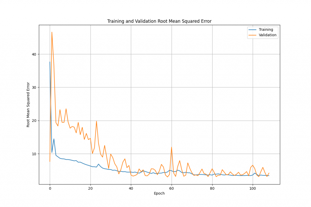
The code to do this (using matplotlib) is quite straightforward:

# Graph the results
training_loss = history.history['loss']
validation_loss = history.history['val_loss']
 
epochs_range = range(len(history.history['loss']))
 
plt.figure(figsize=(12, 8))
plt.grid(True)
plt.plot(epochs_range, 
         [x ** 0.5 for x in training_loss], 
         label='Training')
plt.plot(epochs_range, 
         [x ** 0.5 for x in validation_loss], 
         label='Validation')
plt.xlabel('Epoch')
plt.ylabel('Root Mean Squared Error')
plt.legend(loc='upper right')
plt.title('Training and Validation Root Mean Squared Error')
plt.savefig('{}/{}_rmse.png'.format(output_path, output_name))
plpy.notice('Created: {}/{}_rmse.png\n'.format(output_path, 
                                               output_name))

We first grab the training and validation loss values for each epoch from the history object that the model.fit() method returned. We figure out the range of epochs to plot along the X axis, set up to create a basic plot, and then add the two series (square rooted, so we can compare the numbers with the actual data). Finally, we set up legends and labels etc. and save the image.

At this point we have a saved model that we can load as needed to perform analysis on new or hypothetical data. We can also re-train 'on top' of that model if we get new data that we want to use to improve it.

You will remember that earlier we created a set of test data in addition to our training and validation data sets. At this stage we can use the model.evaluate() method, passing it the test input and output features in order to further test the model. It will run predictions in test mode and return loss and metrics values to indicate how well the model performed.

 

Performing Analysis

Actually using the model we've created to perform analysis is quite straightforward and can easily be wrapped up into a general purpose pl/python3 function:

CREATE OR REPLACE FUNCTION public.tf_predict(
    input_values double precision[],
    model_path text)
  RETURNS double precision[]
  LANGUAGE 'plpython3u'
  COST 100
  VOLATILE PARALLEL UNSAFE
AS $BODY$
import tensorflow as tf
 
# Reset everything
tf.keras.backend.clear_session()
tf.random.set_seed(42)
 
# Load the model
model = tf.keras.models.load_model(model_path)
 
# Are we dealing with a single prediction, or a list of them?
if not any(isinstance(sub, list) for sub in input_values):
   data = [input_values]
else:
   data = input_values
 
# Make the prediction(s)
result = model.predict([data])[0]
result = [ item for elem in result for item in elem]
 
return result
$BODY$;

First, we define the SQL interface to the function, passing in an array of input features, and the path to the saved model.

Within the function body, we import the TensorFlow library, and then ensure that everything is reset. The model is then loaded from the path given.

We can use the function to make one or multiple predictions at once, by passing in either a one dimensional array of input features, or a two dimensional array containing multiple sets of features. TensorFlow is expecting a two dimensional array (actually, a list of lists or similar objects such as Numpy arrays or TensorFlow tensors), so if we only pass in a one dimensional array, we need to change that into a list containing a single list of the features. Otherwise, we leave it as-is, as PostgreSQL will have already converted a two dimensional array into a list of lists for us.

The model.predict() method is then used to analyse the data and make predictions, and returns a Numpy array of results which we convert into a list and return to PostgreSQL. The function can be seen in use below:

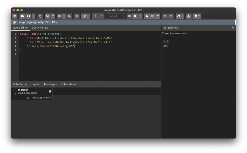
This example uses two rows that I picked randomly from the Boston Housing dataset (because we know what the result value for them should be). I removed the three columns that were most loosely correlated to the medv column (chas, dis and b) and then trained a model with four layers of 64 filters in addition to the input and output layers, over 5000 epochs (early stopping occurred at epoch 108).

 

Conclusion

In this blog mini-series, we have explored how to setup PostgreSQL so that we can use TensorFlow from within our databases, how to examine and optimise data for training a model, and then how to perform the training and use the model to make predictions.

It can easily be seen that the techniques shown here offer a huge amount of possibilities; the use of TensorFlow with pl/python3 is almost just an example, albeit a very powerful and interesting one, but of course similar code can be used with other machine learning libraries such as PyTorch, or in fact, any other libraries that could be used to do interesting things with data in PostgreSQL.