180x Faster Recovery: How EDB Postgres® AI Rewrote RPO/RTO Math with WarehousePG Disaster Recovery

A banking customer relying on logical backups had developed several serious problems over time they could no longer ignore: A full backup took nearly two days to complete. This warehouse is the home to hundreds of terabytes of business-critical data—and let’s not forget the domain knowledge and decades of business logic—and it had to be online 24x7. Backups ran nearly every hour of every day. Restoring to their disaster recovery (DR) cluster took just as long.

The DR policy called for a two-hour recovery point objective (RPO) and recovery time objective (RTO), meaning a 24x gap between what the business required and what the tooling could deliver. That’s not the kind of gap you close with more process, discipline, or a longer maintenance window. A pivot of tooling was required.

To put it plainly: If that cluster had gone down, the business would have lost up to two days of data and spent two more getting it back. For a platform holding customer, transactional, and operational data at the center of a 24x7 analytics pipeline fueling daily decision-making, that isn’t an inconvenience. It’s an unhedged risk sitting quietly on the books, until the day it isn’t quiet anymore.

Today that same cluster recovers to a point within the last 15 minutes—a roughly 180x improvement in both RPO and RTO—with no changes to the application architecture that sits on top of it. This is the story of how and, more important, what it actually took to get there with EDB Postgres AI.

Who needs to read this

Not every deployment needs what I will describe here. This is written for teams for which at least one of the following is true:

• You operate in a regulated industry and RTO and RPO aren’t aspirational. There’s a third-party audited process, and a missed target is not a footnote.

• Your ELT pipelines run continuously. If a long backup causes data to pile up, you can’t just press “replay” to catch up.

• You run high-concurrency or HTAP workloads, so a backup process competing for locks and I/O shows up immediately as degraded query performance for real users.

• Your deployment has quietly become “too big to back up,” or, as I told the customer, they were “a victim of their own success.” The backup tooling that worked at 10 terabytes has stopped working at 80x the volume.

• You’re not doing backups today at all, for whatever reason—infrastructure gaps chief among them. The absence of a plan has itself become a risk.

• You need to reduce your IT budget through consolidation of workloads running on one or many expensive solutions into an affordable, fixed-price solution requiring a DR plan.

If none of that describes your environment—you’ve got a small deployment, or a dev/test system for which a few hours of data loss is a shrug rather than an incident—this is still useful background. But the urgency described here won’t feel like yours yet. For everyone else, keep reading.

Defining the problem

Scale doesn’t ask permission. As table counts, data volume, and concurrency grow, backup tooling either scales with them or becomes the bottleneck itself.

Logical backups have to freeze the world first. To guarantee that schema and data reflect one consistent moment, every table takes an ACCESS SHARE lock, enough to block a DROP TABLE or TRUNCATE and enough to guarantee a clean snapshot.

At hundreds of thousands of tables and hundreds of terabytes, that lock isn’t free. It queues. It bloats the catalog. At the extreme, it exhausts the lock table resulting in the message:

ERROR: out of shared memory

HINT: You might need to increase max_locks_per_transaction.

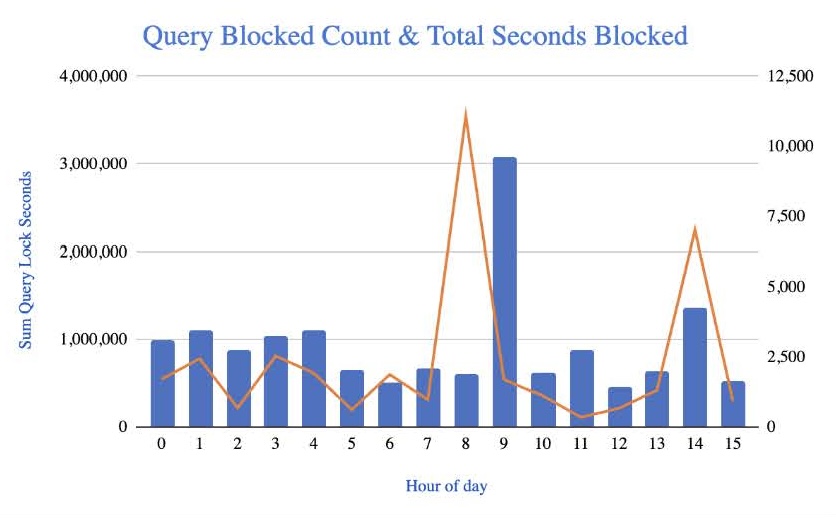
This is what that looked like in practice: real queries, stacked up behind a lock they never should have had to wait on. It was the customer's reality. Breaking the whole backup into smaller backup sets focused on an applications schema (or group of) offered little relief. Backups were still running nearly every hour of the day.

The cost isn’t abstract. It’s missed SLAs, second-guessed SLOs, ELT pipelines falling behind schedule, and a user experience that quietly degrades every time the backup job runs.

Simply switching to volume snapshots is not a solution. In an MPP cluster, “consistent” doesn’t mean one node. It means the coordinator and every segment agreeing on the same point in time, simultaneously. That’s a harder problem than single-node Postgres backup ever had to solve, and it’s exactly where infrastructure solutions fall down first.

Keep reading. The graph above is the day of cut-over to whpg-dr up to when logical backups were turned off.

Planning

Core discovery

How did I get there? Through planning, discovery, and more planning. What it comes down to is four necessary data points to create the DR plan:

• Network attached storage (NAS) capacity and capabilities or cloud storage budget constraints

• Cluster primary segment size less log files during the planned full backup window

• Database activity measured in write-ahead log (WAL) files produced per day for all segments

• And, finally, an average WAL compression

   

NAS storage capacity is, of course, critical to success. However, capabilities including deduplication and compression can greatly increase retention. Deduplication also commonly benefits the backup process itself, reducing data sent. Many solutions exist with this capability, and I cannot emphasize enough the importance of their features. A full backup of 200 TB historical data taking 10 hours to complete can quickly become only 2 TB and 30 minutes with the right solution. I cannot say enough good things about cost efficiencies in deduplication.

Regarding the deployment that is the focus of this article, it was in the cloud, so really an object storage, cost optimization, and budget question. Amazon S3 Standard — Infrequent Access or Google Cloud Storage Coldline are both priced well for the purpose.

WarehousePG mirror segments are not backed up; only primary segments are. Estimating database size becomes a simple \l+ command in psql and total the used column of all logical databases in the cluster. Alternatively, use gpssh -f segment_hosts "df -h /data1 /data2" replacing the data volumes with those in your cluster, total the used column, and divide by two. This method will be a rough estimate, as a full backup does not include the log/ directory. 

WarehousePG, like any other PostgreSQL derivative, records all database modifications to WAL files. Since these are critical for DR, all are archived. No one WAL file can be missing, else the archive is invalidated. Once per hour, schedule a job recording pg_catalog.gp_stat_replication. Using this information may give you a deeper appreciation for what your cluster accomplishes on an hourly basis. 

Script to schedule using cron:

#!/bin/sh

. /usr/edb/whpg7/greenplum_path.sh

psql -qAt -d mydatabase -U gpadmin -c "INSERT INTO myschema.wal_tracking SELECT now(),* FROM pg_catalog.gp_stat_replication;"

Tracking table snapshotting current WAL location and other bits:

CREATE TABLE myschema.wal_tracking (

 period           timestamptz DEFAULT now(),

 segment_id       integer,

 pid              integer,

 usesysid         oid,

 usename          name,

 application_name text,

 client_addr      inet,

 client_hostname  text,

 client_port      integer,

 backend_start    timestamp with time zone,

 backend_xmin     xid,

 state            text,

 sent_lsn         pg_lsn,

 write_lsn        pg_lsn,

 flush_lsn        pg_lsn,

 replay_lsn       pg_lsn,

 write_lag        interval,

 flush_lag        interval,

 replay_lag       interval,

 sync_priority    integer,

 sync_state       text,

 reply_time       timestamp with time zone,

 spill_txns       bigint,

 spill_count      bigint,

 spill_bytes      bigint,

 sync_error       text

) DISTRIBUTED RANDOMLY;

An hourly summary measuring activity in WAL files:

SELECT period, sum(wal_files_per_hour)

  FROM (

SELECT segment_id, period

     , pg_catalog.pg_wal_lsn_diff(

        sent_lsn,

        LAG(sent_lsn) OVER (PARTITION BY segment_id ORDER BY period)

       ) AS wal_files_per_hour

  FROM myschema.wal_tracking

 ORDER BY segment_id, period

) x

 GROUP BY period

 ORDER BY period;

Now, armed with this information, you can determine whether your backup and archive retention requirements are realistic. Answer these questions:

• Is more storage required in your data center?                                                                
• If using cloud storage, does your budget need adjustment?                                                                
• Does your full backup schedule need to be more frequent, or is there room to permit less frequent backups?                                                                

Restore points

The last items worth mentioning on the backup side of the equation are restore points. A restore point is an agreed-upon point in time when the database is consistent. In application and practice, it’s a CHECKPOINT and a gathering of all primary segment LSNs (Log Sequence Numbers) recorded in a file and placed in the archive.

We implemented an hourly restore point. The platform and application permitted full replay ability of all incoming data feeds and analytic jobs. Restore points are cheap from a process and storage standpoint. Creating as many as you like is as simple as a one-line cron job and scheduled once an hour or every five minutes.

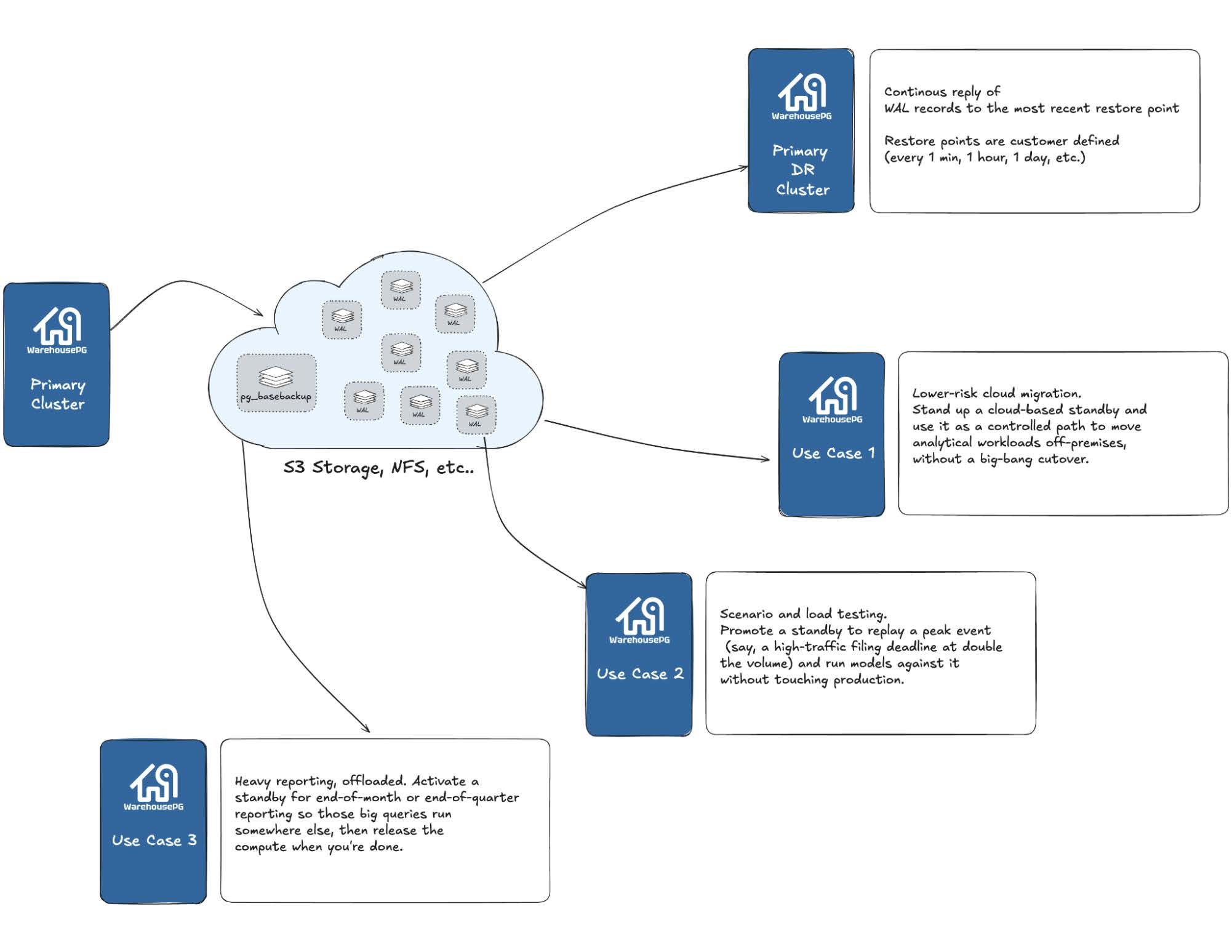
Restore points bring to the surface all of the potential use cases of the Disaster Recovery for WarehousePG utility beyond simple DR. 

• Restore the cluster to just after the books closed for a month or quarter, to offload heavy end-of-period reporting.

• Create a copy of production for QA and performance testing purposes.

• Migrate the cluster from one environment to another, be it cloud or on-premise.

Recovery cluster

No DR plan is complete without testing recovery. Hybrid cloud environments have greater resource constraints compared to the cloud’s near infinite object storage and compute. However, hybrid attached storage will always beat cloud on disk throughput and long-term cost—too bad, since neither really play a role in recovery.

What is worth measuring is WAL replay time. This is the time necessary to fetch a WAL file from the archive, uncompress, and replay it.

Segment logs will be your guide. With some clever scripting focusing on archive fetch entries and measuring the time between current and previous, you will find the magic average-time-to-replay metric. Spoiler alert (having done this many times now): The average is going to land between 0.75 and 1.1 seconds. The differentiating factors will be network latency between archive location and DR cluster and the contents of the WAL file itself. In other words, you have control over the former, not the latter. Contents of the WAL must be replayed. Period.

Why measure WAL replay time? In an acronym, RTO, but better by example. Given a DR cluster that must be no more than one hour behind, there is a finite amount of time to replay WALs. Average WAL replay time will guide you in selecting a minimum replay frequency to match your RTO as well as determine how much headroom you have when someone runs a CTAS with a Cartesian JOIN creating a WAL tsunami. You know it’s happened; don’t even pretend it didn’t.

Results

tl;dr

These are actual numbers from this one deployment. I’ve done a few now and my methodology hasn’t changed much, though my scripts are a ton better! Thanks, Claude!

• 595 TB database reduced to approximately 160 TB

• 1.29 PB WALs / week produced

• 99% (rounded) reduction of query lock times

• 11-hour full backup, down from 44 hours

• DR cluster on small compute instances (cost optimization)

• Hourly restore points replays at, on average, 16 minutes

• Cloud deployment with no deduplication (just a reminder)

WAL by the numbers

What we discovered surprised us. Graph is the maximum WAL production per hour over the source of one month. The maximum expected WALs for any 24-hour period is just under 8M, or 484 TB uncompressed. We experienced an average compression of 3:1, reducing to 161 TB. Still a significant size when you consider the retention policy target was seven days. Average hourly WAL production was 5M, give or take 10% depending on the hour of the day.

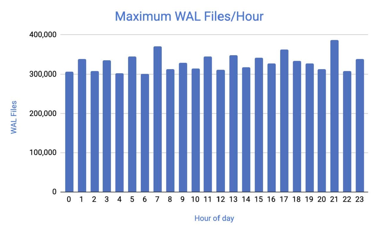
In reality, we kept eight days to allow for the next full backup time to complete, so there was always a full and replayable backup. We also implemented a lifecycle retention policy in the cloud storage to remove objects over eight days old. That’s 1.29 PB of WALs. Far more efficient.

Full backup

You may say, “Greg, what about time to take a backup?” I didn’t forget, nor am I concerned. Physical file system backup requires far less to accomplish than logical. Everything that needs to be avoided is:

• Append-optimized column oriented (AOCO) tables do not have to be materialized into rows.

• Operating outside of the database requires no locks.

• There’s no query overhead, since every table dump is a copy of a file, not a SELECT.

• Indexes, while not uncommon, typically are not used, so that load is minimal.

What once took nearly 44 hours to complete with logical backup utilities became 11 hours 9 minutes and 4 seconds. Resource consumption naturally increased during the backup, but nowhere near the way the old backups did.

• Storage wasn’t stressed with an estimated 22% increase in utilization—lower than that observed using logical backup.

• CPU utilization rose a mere 5%, due only to compression.

• The increase in memory used was so little that I didn’t log it.

• Network transmits increased but never hindered production queries.

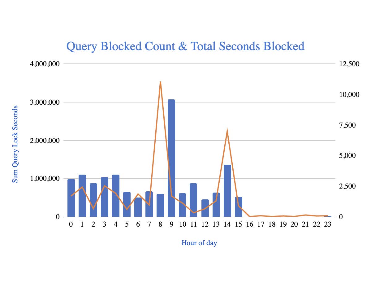
The graph above shouldn’t just grab your attention—it should snap you right out of complacency. It illustrates the day logical backups were turned off in the 15th hour and whpg-dr took over. Average seconds of queries blocked by a lock dropped by 98.86260811%.

Recovery cluster

No DR plan is complete without testing recovery, and this is the metric that actually matters when the pager goes off: WAL replay time.

Measuring it takes a little scripting: Isolate archive-fetch entries from segment logs and time the gap between consecutive fetches. Having done this a few times now across on-prem, AWS, and GCP, I can say that the average lands between 0.75 and 1.1 seconds. Split the difference: Call it 0.9 seconds per WAL file, start to finish—fetch from archive, uncompress, replay.

That number holds remarkably steady across environments, and that consistency tells you something useful: Replay is bound by fetch-and-uncompress overhead, not raw compute. It’s why the DR cluster runs comfortably on smaller, cost-optimized instances rather than as a mirror of production-grade hardware. You’re not asking it to do production’s job, just to catch up fast.

Run the actual numbers and it holds up: Across 192 primary segments producing roughly 5M WAL files a day, that’s about 1,085 WAL files per segment in an average hour. At 0.9 seconds each, replaying a full hour’s worth of changes takes about 16 minutes—against a two-hour requirement, that’s better than 7x the headroom the business asked for.

That’s the whole point of hourly restore points: Recovery isn’t an overnight project, it’s a coffee break.

Conclusion

Real credit here belongs to the engineering teams behind the tools: both WarehousePG and Barman. Their attention and time spent testing, retesting core functionality, and edge cases resulting in a product that coordinates backups and continuous WAL archiving across a petabyte size distributed cluster is amazing. All of that capability bundled up into a utility that is simple and elegant, and done in relatively short order: a notably faster time-to-market than the industry has seen for comparable point-in-time recovery (PITR) capability elsewhere.

What it doesn’t do for you is your planning. Measuring WAL volume, right-sizing storage, validating storage capabilities, selection of a compression algorithm, deciding how many restore points you can afford…. All that is discovery and discipline that has to happen before you ever flip the switch, and no utility does it for you.

I hope this article was instructive, and when you make the move to EDB Postgres AI for WarehousePG, just remember what is on the other side with whpg-dr:

• Two days to 16 minutes. 

• Forty-four hours to 11.

• A 99% drop in lock contention. 

• None of it touched the application.

The technology already existed—PITR has been part of Postgres for years. What changed was the discipline to plan for it properly before flipping the switch.

No longer is there any reason to not have a DR plan.

For full installation and configuration instructions, documentation can be found in EDB’s public documentation.